Quantum computers are all the rage lately, but what even is a quantum computer? And why do we need them?
In the first part of this series we saw how we can encode information in a way that classical computers can work with it, and how they process this information. We also defined what ‘algorithm’ means and introduced the notion of a randomized algorithm. Lastly, we presented different ways in which a computer can be realized physically.
In this second episode, I will talk about quantum computers. We will see the very basics of quantum mechanics and then I will translate all the ideas explained for classical computers to the quantum domain: we will see how to encode information in a quantum way and how to manipulate it. To finish, I will briefly justify why quantum computers are interesting and might prove useful in a not too distant future.
Quantum computers are computers in the sense that they process information: they take some input and produce some output. The difference with classical computers lies in the rules they follow – rules that are inspired by quantum mechanics. Therefore, before talking about quantum computers, we are going to introduce a few concepts of quantum mechanics.
Basics of quantum mechanics
Warning: this section is by no means an explanation of quantum mechanics – it is not even a good introduction to it. It is essentially a list of statements that you should take at face value – don’t overthink it!
We will call our object of study “the system” and each configuration of the system “a state of the system” or just “a state”. The system is in some state, and to extract information from it we have to measure it. This is just like in classical mechanics: a ball flying through the air will be in some state: it will have some position and some velocity. To know them, you have to make a measurement.
To perform any measurement, we use some measuring device such as a ruler for length, a scale for weight… Mathematically, this measuring device is often assumed to be perfect, but physically it will have imperfections and limitations. Nevertheless, note that according to the most popular views the facts in the following paragraphs are independent of the physical device: they are not an artefact of the specifics on the construction of the device, but an intrinsic part of nature.
We can calculate the state of the system at any given time (provided we specify its initial conditions), but when we measure it we can only observe it in some specific states. Perhaps an analogy is enlightening: imagine you had a magical compass that could be pointing in any direction and you could calculate where it is pointing at at any given time once it has been prepared in a certain way. But when you looked at it you could somehow only see it pointing either north or east – the measurements only give you partial information about the exact state
Let’s call the set of states that can be observed the “observable states”. Suppose the system can only be in 4 observable states that we call \(A, B, C, D\). Any ‘true’ state of the system can be expressed as a combination of the observable states. For example, the following are valid states of the system:
\(\begin{align*}
C, \quad 0.64 A – 0.3 B + 0.63 C + 0.32 D, \quad -0.6 A + 0.8 C, \quad 0.3 B + 0.9 C + 0.32 D.
\end{align*}\\
\)
If the system is in a state which is the sum of more than one observable state, such as in the last 3 examples, we say it is in a superposition of those states.
In general, the state of the system can be written as
\( \alpha_1 A + \alpha_2 B + \alpha_3 C + \alpha_4 D, \\\)with \(\alpha_1,\alpha_2, \alpha_3, \alpha_4\) numbers called probability amplitudes. \(\alpha_1\) is the probability amplitude of A, \(\alpha_2\) is the probability amplitude of B, and so on.
When we observe the system, we can only see it in either state \(A\), or \(B\), or \(C\), or \(D\). The probability that we observe it in A is1 \(|\alpha_1|^2\), the probability that we observe it in B is \(|\alpha_2|^2\), for C it is \(|\alpha_3|^2\) and for D it is \(|\alpha_4|^2\). In this way, the probability amplitudes tell us how likely it is that we observe the system in a specific observable state. And therefore, \(|\alpha_1|^2 + |\alpha_2|^2 + |\alpha_3|^2 + |\alpha_4|^2 = 1\), as the sum of the probabilities of all outcomes has to be 1. Note that in the examples above, the probabilities indeed add to 1 – of course, up to rounding errors.
After the measurement, the system “remains” in the state in which we observed it. We say it collapses to that state.
Going back to the made-up example of the compass, we would say it only has 2 observable states: \(N\), corresponding to it pointing north, and \(E\), corresponding to it pointing east. And when it is in your pocket, it can be in a superposition of \(N\) and \(E\) – for instance, in the state \(0.4 N + 0.92E\). This means that when you take it out of your pocket and “measure” it by looking at the needle or by taking a picture with your phone (measuring doesn’t necessarily mean that a sentient being is observing it through its senses), the measurement will report ‘north’ with probability \(|0.4|^2 = 0.16 = 16\%\) and ‘east’ with probability \(|0.92|^2 = 84\%\). Consequently, the compass’ state will collapse (be updated) to north with probability \(16\%\), or to east with probability \(84\%\).
As long as we do not measure the system, it will evolve in time according to an equation known as Schrödinger’s equation. The compass could at one instant in time be in the state
\( 0.707N + 0.707E,\\ \)and then after some time in the state
\( -0.02N+0.9998E.\\ \)If you had observed it at the first moment, the probabilities would have been
\(
\begin{align*}
\text{prob}(N) &= |0.707|^2 = 50\%, \\
\text{prob}(E) &= |0.707|^2 = 50\%,
\end{align*}\\
\)
and now they have become
\(
\begin{align*}
\text{prob}(N) &=|-0.02|^2 = 0.04\%, \\
\text{prob}(E) &= |0.9998|^2 = 99.96\%.
\end{align*}\\
\)
For any quantum system the evolution in time is perfectly determined. There is no randomness to it, it is deterministic, and it is determined by the “forces” acting on the system. Therefore, we can act on the system to dictate its evolution and influence with which probability each possible outcome can be observed.
A classical picture might help clarify the idea: consider a fair die spinning in the air randomly. We don’t know on which face it will land, but we know the probability of observing each face: 1/6. If before it lands we nudge it in an adequate manner (a force acts on the system), we can make it rotate around an axis perpendicular to two of its faces (the faces 2 and 5 in the drawing). We still do not know on which face it will land, but we know that the probabilities have changed: it is now impossible that it lands on faces 2 and 5, so they have a probability of 0, and the rest of the faces have a probability of 1/4.
A different example: if you had the special ‘quantum compass’ in your pocket, it might be in a state such that when measured it could give every possible outcome with the same probability. But if, without looking at the compass, you place a magnet towards the east, the state of the compass will change to one where it is very likely that you observe the needle pointing east.
Quantum computing
Now that we know what rules quantum mechanics imposes on us, we can understand how to use them to our advantage and perform computations within the quantum mechanical framework.
In quantum computing, the goal is to encode the possible answers to a computational problem, including the correct answer, as observable states of a quantum system. As explained, when we measure the system, the outcome will be an observable state and depending on the state of the system, the probability that the outcome is one or another will be different. That implies that measuring the system will give us the correct answer to the problem with some probability which depends on the state of the system. The essence of quantum computing is then to act on the system (before measuring it) in such a way that the probability that we observe the correct answer is maximised and ideally very close to 1.
An example: say a problem has possible answers \(A, B, C,\) but only \(C\) is the correct one. We “generate” a system in state \(0.8A+0.4B+0.45C\) so the probability of observing the correct answer is \(|0.45|\)or roughly 20%. We act on the system, without measuring it, to change its state to \(0.2A+0.1B+0.97C\). Now the probability of observing the correct answer is \( | 0.97| \), roughly 94%.
Qubits
Analogous to a bit in classical computing, the smallest unit of information in a quantum computer is a quantum bit or qubit. A qubit is a quantum system that has 2 observable states that we denote \( | 0 \rangle \) and \( | 1 \rangle \) This notation is called bra-ket notation. Any state our system can be in, can be expressed as a superposition of the two observable states. Thus, the state of a qubit in general is
\( a_0 | 0 \rangle + a_1 | 1 \rangle \)
with \(a_0, a_1\) complex numbers such that \(|a_0|^2+|a_1|^2 = 1\).
If we have a system of multiple qubits, the observable states of the system can be written by joining the observable states of each qubit. For example, for 2 qubits the observable states are \( | 0 \rangle | 0 \rangle , | 0 \rangle | 1 \rangle , | 1 \rangle | 0 \rangle , | 1 \rangle | 1 \rangle \). For 3 qubits: \( | 0 \rangle | 0 \rangle | 0 \rangle , | 0 \rangle | 0 \rangle | 1 \rangle \), etc. – eight observable states in total. Since writing the brackets becomes tedious very quickly, we often abbreviate: instead of \( | 0 \rangle | 1 \rangle | 1 \rangle \) we write \( | 011 \rangle \), instead of \( | 1 \rangle | 1 \rangle | 0 \rangle \) we write \( | 110 \rangle \), and so on.
As usual, the full state of a system of qubits can be written as a superposition of the observable states of the system:
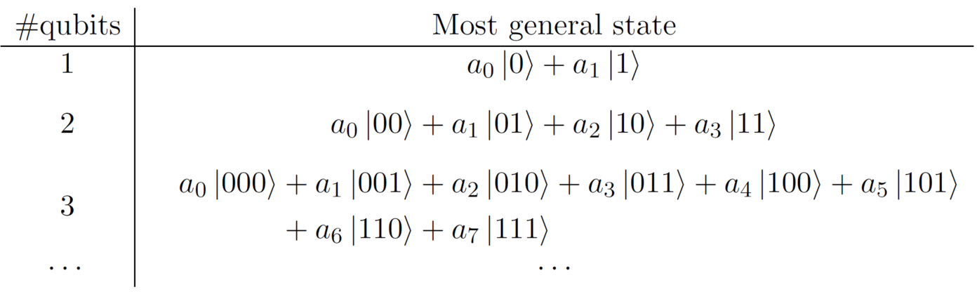
And as usual, the probability that when measuring the system we observe a certain state equals the square of the probability amplitude of that state.
Example: For a system of 3 qubits, the probability of observing \( | 010 \rangle \) is \(|a_2|^2\), and the probability of observing \( | 110 \rangle \) is \(|a_6|^2\ldots\). Since probabilities add to 1, we must have
\( |a_0|^2+|a_1|^2+|a_2|^2+\ldots = 1 \)
When, for example, one qubit is in an observable state and one is in a superposition, we can write the combined state in different ways:
\( | 1 \rangle \left(0.3 | 0 \rangle +0.95 | 1 \rangle \right) = 0.3 | 1 \rangle | 0 \rangle + 0.95 | 1 \rangle | 1 \rangle = 0.3 | 10 \rangle + 0.95 | 11 \rangle \)
Operations on qubits
Acting on the system corresponds to performing operations on its state. For example, the Hadamard operator \(\text{H}\) operates on a single qubit in the following way:
\(\begin{align*}
\text{H} | 0 \rangle &= \frac{1}{\sqrt{2}} | 0 \rangle +\frac{1}{\sqrt{2}} | 1 \rangle \\
\text{H} | 1 \rangle &= \frac{1}{\sqrt{2}} | 0 \rangle -\frac{1}{\sqrt{2}} | 1 \rangle
\end{align*}\\
\)
Note that the coefficients on the right hand side indeed, when squared, still add up to 1. An operation acting on a combination of states operates on each term:
\(\begin{split}
\text{H} \left(0.2 | 0 \rangle + 0.98 | 1 \rangle \right) &= 0.2\, \text{H} | 0 \rangle + 0.98\, \text{H} | 1 \rangle \\
&= 0.2 \left(\frac{1}{\sqrt{2}} | 0 \rangle +\frac{1}{\sqrt{2}} | 1 \rangle \right) + 0.98 \left(\frac{1}{\sqrt{2}} | 0 \rangle -\frac{1}{\sqrt{2}} | 1 \rangle \right) \\
&= \frac{0.2 + 0.98}{\sqrt{2}} | 0 \rangle + \frac{0.2-0.98}{\sqrt{2}} | 1 \rangle \\
&= 0.83 | 0 \rangle – 0.55 | 1 \rangle
\end{split}\\
\)
Note how the probabilities of observing \( | 0 \rangle \) and \( | 1 \rangle \) have changed after applying the \(\text{H}\) operation:
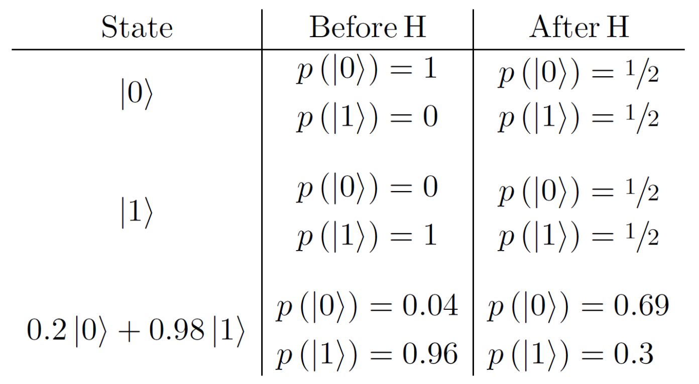
Also note how by applying \(\text{H}\) to \(0.2 | 0 \rangle + 0.98 | 1 \rangle \), it has been applied to both \( | 0 \rangle \) and \( | 1 \rangle \) simultaneously. This is an illustration of a general phenomenon which is that, in quantum computing, operations act on all states of a superposition at once. Contrast that to the classical case, where if we wanted to apply some logical gate to multiple states, say an AND gate, we needed to apply it to them one by one: 0 AND 0, 1 AND 0, … This affords quantum computers a sort of parallelism that classical computers do not enjoy.
In a system of more than a single qubit, each operation acts on some of the qubits of the system. There are operations that act on all of the qubits, operations that act, say, only on the 2nd one and the 7th one, operations acting only on the last qubit, and so on.
Example: Consider a system of 3 qubits with \(\text{H}\) operating only on the 2nd one:
\(\begin{split}
\text{H} _{(2)} | 011 \rangle &= | 0 \rangle \text{H} | 1 \rangle | 1 \rangle \\
&= | 0 \rangle \left( \frac{1}{\sqrt{2}} | 0 \rangle -\frac{1}{\sqrt{2}} | 1 \rangle \right) | 1 \rangle \\
&= \frac{1}{\sqrt{2}} | 001 \rangle – \frac{1}{\sqrt{2}} | 011 \rangle
\end{split}\\
\)
Lastly, we can think of measuring the system as applying a special operation to it, the output of which is one of the observable states. Note that we do not need to measure all qubits at the same time, so also this operation can be applied to a subset of the qubits.
After measuring, we interpret the observed state as a bitstring of classical bits. For instance, if the output state after the measurement is the observable state \( | 001 \rangle \), we understand the output of the computation to be \(001\).
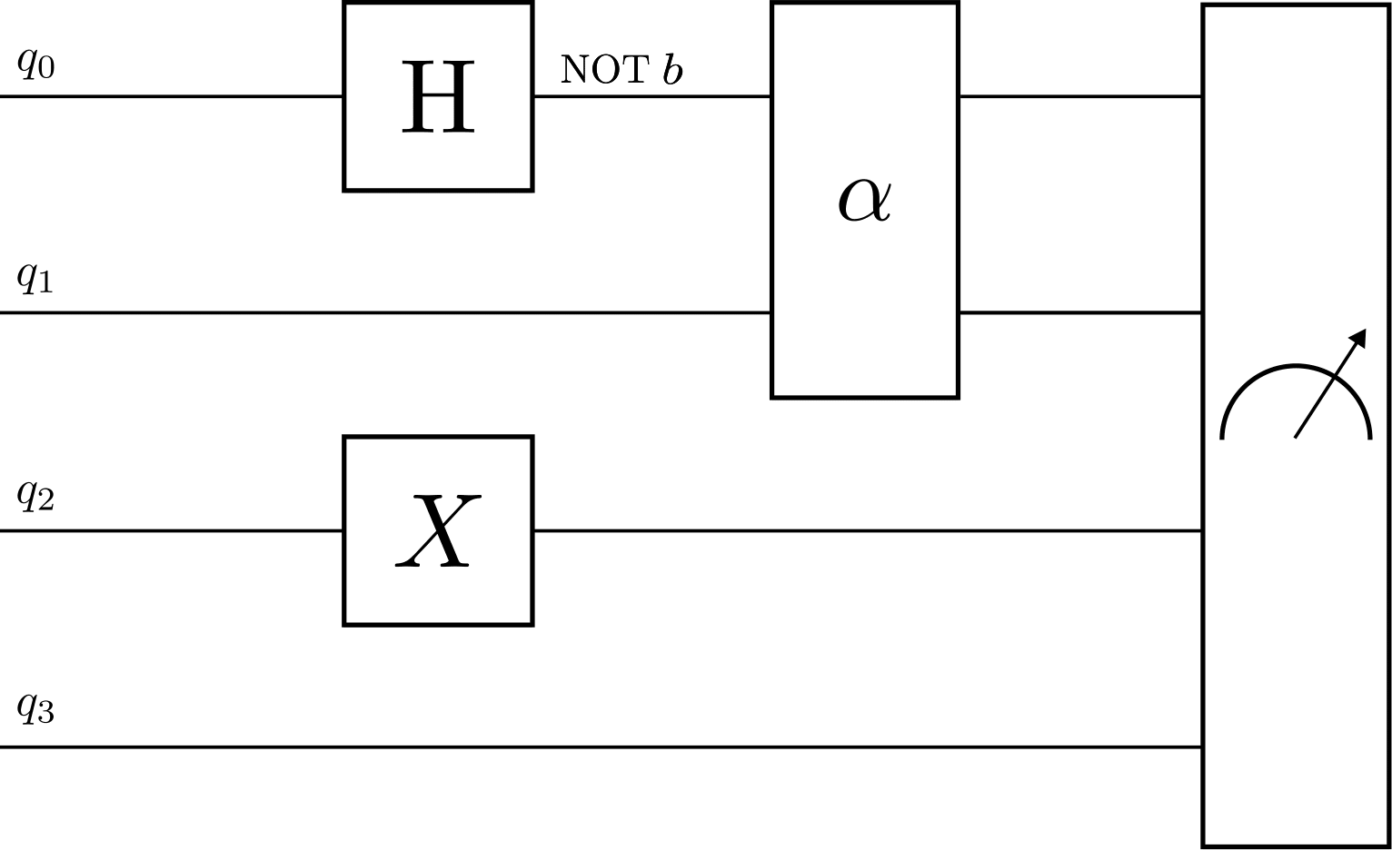
As with classical computers, we call the successive application of operations on a state a (quantum) algorithm. Similarly to what we saw in the previous article for ‘classical’ algorithms, quantum algorithms can also be represented in a diagram with each line being a qubit, each box an operation on its input qubits and time flowing left to right.
Repeating what I said in the introduction of this section, but using the new terminology introduced: quantum computing is about applying operations to a system of qubits so that the probability of observing the state corresponding to a correct answer to a problem is maximised.
Why quantum computers?
Given that we already have extremely fast and reliable computers, a fair question to ask is: why go through all the hassle of qubits and quantum gates to perform computations? Can’t we just use classical computers? Here I will present two out of many arguments that hopefully illustrate the need for quantum computers and their advantages.
First, suppose we want to study a system of qubits with a classical computer. Recall that the general state of the system for different amounts of qubits is
Thus, for one qubit we need to store \(a_0\) and \(a_1\), two numbers. For two qubits, we store \(a_0\) up to \(a_3\), four numbers. For three qubits we must store eight numbers. And the pattern continues: for 4 qubits, 16 numbers; for 5 qubits, 32 numbers, multiplying by two every time a qubit is added. In general, for \(n\) qubits, the amount of numbers needed is \(2^n\). Assuming there are \(10^{80}\) atoms in the universe (the Eddington number) and assuming we can store one number per atom, then using the entire universe we could simulate a system of a grand total of \(n = 266\) qubits – a tiny amount! This example, while not completely accurate2, illustrates that if we want to study a quantum system such as a large molecule, we are very limited by classical computers. If, for example, we wanted to keep track of the position of each atom in the molecule, we would quickly run out of memory. Nevertheless, with a quantum computer we would not need to store the information describing every atom in the molecule, we could just simulate the interactions between the atoms in the molecule and study the properties of this “artificial” molecule.
Second, quantum computers are fundamentally different in the way they operate, which allows for faster algorithms. The operations that quantum computers perform are not just faster classical operations, they are different. For instance, a classic gate only acts on 1 state at a time. Whereas a quantum gate, in a way, acts on all possible states of the system simultaneously. For instance, an area where this property of quantum computers offers the possibility of faster computation is transportation and logistics. Suppose we wanted to find the optimal route connecting two cities to transport some freight – maybe we wanted to find the shortest route, maybe the fastest, the most fuel efficient… A classical computer would need to check every possible route one by one and compare them, whereas a quantum computer could, in a way, check all of the possible routes in parallel and find the optimal one much faster.
Summary
Computers process information, but they do so in different ways. In this series, we have seen two paradigms of computing: classical and quantum.
In a classical computer, discussed in the first part of the series, the smallest unit of information is the bit, a system that can be in one of two states: 0 and 1. We can encode information such as images or numbers as strings of bits. We manipulate bits by applying logic gates to them. And we can construct algorithms: circuits of logic gates that perform complex operations on strings of bits, that correspond to some kind of information manipulation that we are interested in – for instance, performing mathematical operations.
Quantum computers, discussed in this second part, process information according to rules inspired by quantum mechanics. In a quantum computer, the smallest unit of information is the qubit, a quantum system that can be in a superposition of two states: \( | 0 \rangle \) and \( | 1 \rangle \). A system of qubits will evolve in a way that we can predict but, when measured, it will collapse randomly to one of the observable states. Quantum computing is about encoding an answer to a problem as one of the observable states of a system of qubits, and then manipulating the system in such a way that the probability that it collapses to a correct answer when observed is made as large as possible.
Quantum computers are not just fast classical computers, they are fundamentally different. This enables them to perform certain tasks substantially faster than classical computers, or to even tackle problems that are classically intractable due to their size. Will the quantum computer change the world in much the same way that the classical computer did? Only time can tell!
[1] In fact, a probability amplitude can even be a complex number, in which case the probability is the square of its absolute value. In this article, we will not need this technical detail, but keeping this in mind we will later write the squares with absolute value bars: \(|x|^2\).
[2] See Ronald de Wolf’s lecture notes on quantum computing, section 13.3.
Alle artikelen in deze serie:
- DRESDYN: From science to society
- Cosmic shower
- Wanted: intermediate mass black holes
- Cross sections and higher dimensions
- Why relativity needs a quantum makeover
- Computing: from classical to quantum (1)
- Computing: from classical to quantum (2)
- On the simulation of our reality
- How to find invisible stuff