Quantum computers are all the rage lately, but what even is a quantum computer? And why do we need them?
Introduction
Computers are ubiquitous. You are probably reading this on one and I bet there are at least two in the room where you are. We use them all the time and for extremely complex tasks such as simulating the combustion of gases inside rocket engines, discovering new medicines or watching 5 minute cooking videos. However, it seems like they are not powerful enough. For instance, the simulation of fluid flow over such a simple shape as a flat surface is still only possible to run on world-leading supercomputers.
Lately, we constantly hear about quantum computers, a new kind of “magical” computers that will make current ones seem as fast as a snail next to a fighter jet. But what even is a computer? And what makes quantum computers so special? In this set of articles I give an introduction to the mathematics of computing, both classical and quantum, in an attempt to make more precise what we mean by computing and to demystify quantum computing.
Bits and information encoding
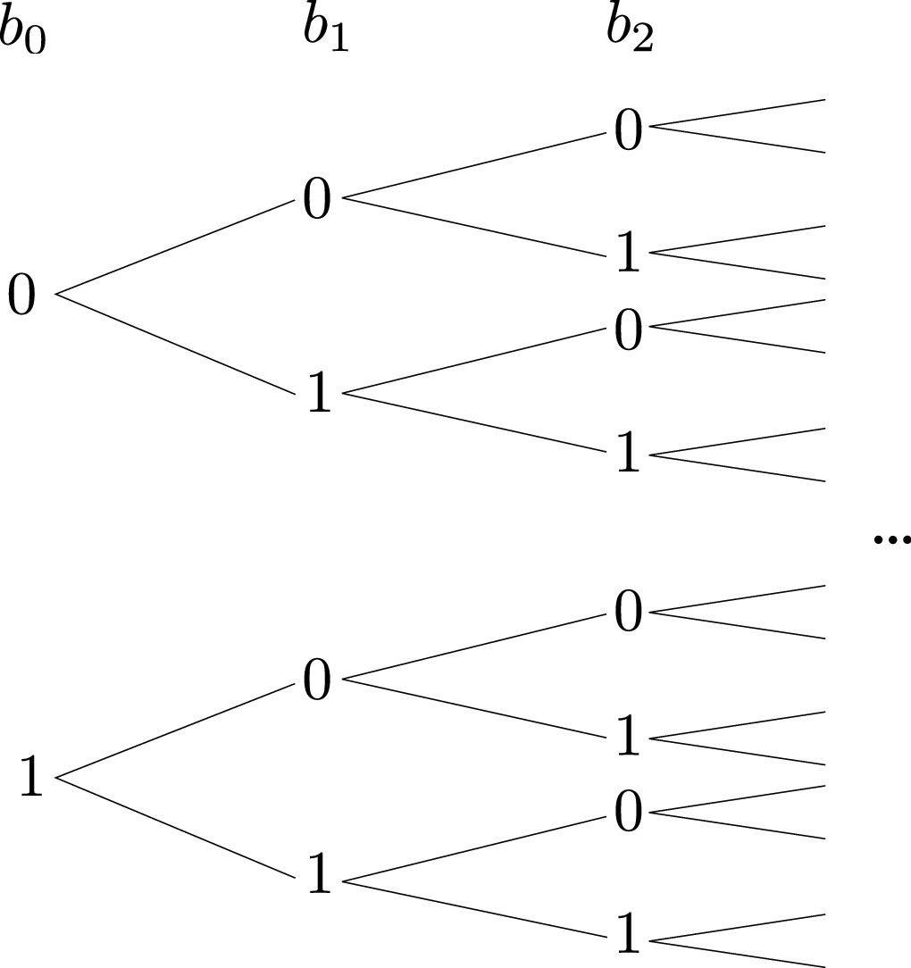
Intuitively, we think of a computer as a box that processes information: it takes some input and produces some output. In classical computing, the smallest unit of information is the bit. A bit can be in one of 2 states that we call 0 and 1. For many bits, their possible collective states are just the combination of the individual states of each bit. If we have a string of 2 bits, that we call \( b_0 \) and \( b_1 \), the only possible states of the string are: \( b_0 = 0 \), \( b_1 = 0 \) or \( b_0 = 0 \), \( b_1 = 1 \) or \( b_0 = 1 \), \( b_1 = 0 \) or \( b_0 = 1 \), \( b_1 = 1 \). For 3 bits, the only possible states are \(b_0 = 0\), \(b_1 = 0\), \(b_2 = 0\) (which we simply write as \( 000 \)), or \( 001 \), \(010\), \(011\), \(100\), \(101\), \(110\), \(111\). And so on.
We can encode numbers into bit strings – for instance, by encoding each number into its binary representation:
\( \begin{array}{ll}0 \rightarrow 0 & 3 \rightarrow 11, \\
1 \rightarrow 1 & 4 \rightarrow 100, \\
2 \rightarrow 10 & 5 \rightarrow 101.
\end{array}\\
\)
But we could as well choose some other encoding:
\(\begin{array}{ll}
0 \rightarrow 0 & 3 \rightarrow 111, \\
1 \rightarrow 1 & 4 \rightarrow 1111, \\
2 \rightarrow 11 & 5 \rightarrow 11111.
\end{array}\\
\)
Information can be encoded into numbers. For example, the alphabet can be encoded as
\(\begin{array}{l}
a \rightarrow 1, \\
b \rightarrow 2, \\
c \rightarrow 3,
\end{array}\\
\)
or a grayscale picture can be encoded in the following way:
In a grayscale picture, each pixel can be completely black, completely white or a gray shade in between. Calling black 0, white 100, we can encode gray shades by ‘how close to black or white they are’.
Since we can encode information into numbers and numbers into bits, we have a way of encoding information into bits, which is what computers work with.
Operations on bits
But how do computers manipulate bits? What kind of operations can they do with them? A typical set of operations a classical computer can do are logic gates: black boxes that take some bits as inputs and output some other bits1. In this section it can help to think of false \(\rightarrow 0\), true \(\rightarrow 1\). The simplest gate, besides that which does nothing on the input, is the NOT gate, which takes one bit as input and outputs 0 if that bit has value 1, and 1 if it is 0. There are many two-bit gates. For instance, there is the AND gate, that takes two bits as inputs and returns in its output bit a value of 1 only if both inputs are 1, and otherwise it returns 0. There is also the OR gate, that takes two input bits and returns 0 only if both are 0, and returns 1 otherwise.
We can write the effect logic gates have on inputs in a table, where the columns represent the values of the input bits except for the last one, that represents the output of the logic gate for the input corresponding to each row:
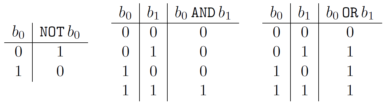
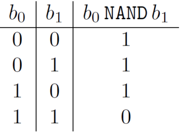
Combining these simple logic gates we can perform more complex operations such as a NAND (NOT AND), which takes 2 inputs and returns an output that is equal to 0 only when both inputs are 1, and equals 1 otherwise, or even addition and subtraction2.
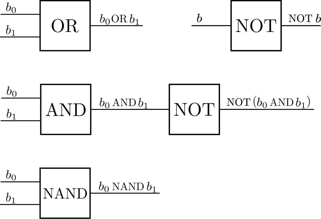
We can represent these operations in diagrams where each line represents a bit and each block is a black box that “performs” an operation on its inputs, with the flow of inputs to outputs going from left to right. For example:
Using multiple gates we can build complex circuits. The output of the whole circuit below is usually compacted into a single gate called XOR (exclusive OR):
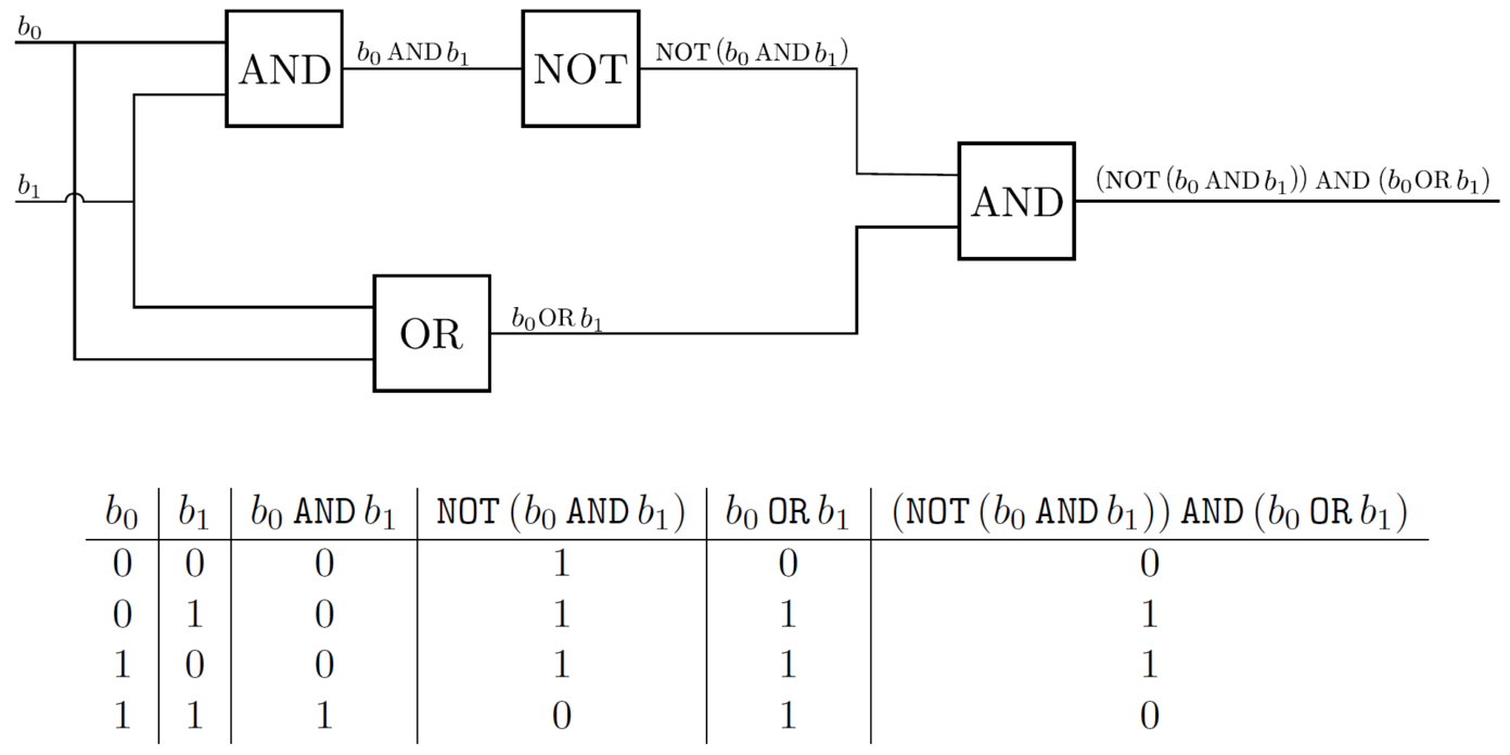
We now have a way to diagrammatically represent the operations that a computer will do to an input in order to obtain an output. Such a set of operations or steps is called an algorithm, and we can picture any algorithm as the diagram of a circuit.
Randomized algorithms
The algorithms presented so far are what is called deterministic: given a particular input, they will always produce the same output, and the intermediate states will also always be the same. However, some algorithms called randomized algorithms employ some randomness in their procedure and may output different answers to the same input.
For instance, suppose we are given an array of \(n \geq 2\) elements (for even \(n\)) in which half are the letter \(\texttt{a}\) and the other half are the letter \(\texttt{b}\). For example: \(\texttt{ab, bababa, abba, babbabaaaabb}\), … We want to find a position in the array that contains the letter \(\texttt{a}\). A deterministic algorithm might be: start at position 1. If the array at that position contains an \(\texttt{a}\), end. If it doesn’t, move to the next position and repeat. On the other hand, a randomized algorithm might be: pick a position at random. If it contains an \(\texttt{a}\), end. If it doesn’t, pick a position at random and check again. For some inputs, the randomized algorithm will be much faster, but for others it will be slower or not even terminate.
For an input such as \(\texttt{bbbbaaaa}\), the deterministic algorithm needs to check the first 5 letters to find an \(\texttt{a}\), while the randomized algorithm might get lucky and start checking at a position where there’s an \(\texttt{a}\), so it might succeed on the first attempt. On the other hand, with a string like \(\texttt{bbbbbbb}\), the randomized algorithm will never end.
Physical realizations of classical computers
So far, we have seen the mathematical idea of how computers work, but how do physical machines carry out these abstract operations? There are many ways to construct a device that can compute logic gates. Here is a list of three using different phenomena for illustration:
Marbles: see “Marble computer OR gate & AND gate Digital Logic” by Masked Marble on YouTube.
Water: see “I Made A Water Computer And It Actually Works” by Steve Mould on YouTube.
Electricity: Consider the following electrical circuit (see this website for reference of electrical symbols):
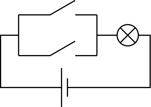
If we close either of the switches, the light bulb will receive electricity and turn on. Considering each switch to represent an input bit, with it being open representing a 0 and it being closed representing a 1, and the lamp to be the output bit, with of course ‘on’ being 1 and ‘off’ being 0, this circuit computes an OR.
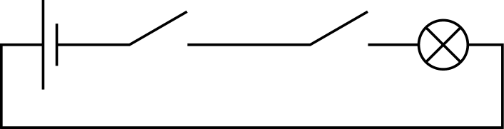
Flipping the switches in a circuit requires manual mechanical action and produces an electrical output. If we could replace these mechanical switches by electricity operated ones, we could chain together outputs of one circuit to inputs of another. These electricity operated switches do indeed exist: they are called transistors and they are the building blocks of current computers3.
Summary
This ends the first part of this series of two articles. We have seen how we can encode information in a way that classical computers can work with it, and how they process this information. We have also learned what ‘algorithm’ means and introduced the notion of a randomized algorithm. Finally, I have presented different ways in which a computer can be realized physically.
In part two, which will appear on 28 June, I will talk about quantum computers. Firstly, we will see the very basics of quantum mechanics and then I will translate all the ideas explained for classical computers to the quantum domain. Stay tuned!
[1] For now, consider logic gates as black boxes. In a later section we will see how they can be implemented in physical computers.
[2] See Sebastian Lague’s video “Exploring how computers work” for examples on how to build circuits that perform useful computations such as the addition of numbers.
[3] For an in-depth video series on how to build a small computer from scratch using electronic components such as transistors, check out the excellent videos by Ben Eater on YouTube.
Alle artikelen in deze serie:
- DRESDYN: From science to society
- Cosmic shower
- Wanted: intermediate mass black holes
- Cross sections and higher dimensions
- Why relativity needs a quantum makeover
- Computing: from classical to quantum (1)
- Computing: from classical to quantum (2)
- On the simulation of our reality
- How to find invisible stuff